Classifying Dogs vs Cats using PyTorch C++: Part 2

In the last blog, we had discussed all but training and results of our custom CNN network on Dogs vs Cats dataset. Today, we’ll be making some small changes in the network and discussing training and results of the task.

I’ll start with the network overview again, where we used a network similar to VGG-16 (with one extra Fully Connected Layer in the end). While there are absolutely no problems with that network, but since the dataset contains a lot of images (25000 in training dataset) and we were using (200x200x3) input shape to the network (which is 120,000 floating point numbers), this leads to high memory consumption. In short, I was out of RAM to store these many images during program execution.

So, I decided to change some minute things:

Input Shape to the network is now 64x64x3 (12,288 parameters - around 10 times lesser than for 200x200x3). So, all the images are now resized to 64x64x3.
Now, we only use 2 Convolutional Layers and 2 Max Pooling Layers to train our dataset. This helps to reduce the parameters for training, and also fastens the training process.

But this comes with a tradeoff in accuracy, which will suffice for now as our target is not to get some X accuracy, but to learn how to train the network on our dataset using PyTorch C++ API.

Question: Does reducing input resolution, affects accuracy? Answer: In this case, it will. The objects in our dataset (dogs and cats) have both high level and low level features, which are visible (provides more details) more to the network with high resolution. In this way, the network is allowed to learn more features out of the dataset. However, in cases like of MNIST, it’s just fine to use 64x64 input resolution as it still allows the network to look at details of a digit and learn robust features.

Let’s go ahead and see what has changed in the Network.

Network Overview

If you don’t remember from the last time, this is how our network looked.

struct NetImpl: public torch::nn::Module {
    NetImpl() {
        // Initialize the network
        // On how to pass strides and padding: https://github.com/pytorch/pytorch/issues/12649#issuecomment-430156160
        conv1_1 = register_module("conv1_1", torch::nn::Conv2d(torch::nn::Conv2dOptions(1, 10, 3).padding(1)));
        conv1_2 = register_module("conv1_2", torch::nn::Conv2d(torch::nn::Conv2dOptions(10, 20, 3).padding(1)));
        // Insert pool layer
        conv2_1 = register_module("conv2_1", torch::nn::Conv2d(torch::nn::Conv2dOptions(20, 30, 3).padding(1)));
        conv2_2 = register_module("conv2_2", torch::nn::Conv2d(torch::nn::Conv2dOptions(30, 40, 3).padding(1)));
        // Insert pool layer
        conv3_1 = register_module("conv3_1", torch::nn::Conv2d(torch::nn::Conv2dOptions(40, 50, 3).padding(1)));
        conv3_2 = register_module("conv3_2", torch::nn::Conv2d(torch::nn::Conv2dOptions(50, 60, 3).padding(1)));
        conv3_3 = register_module("conv3_3", torch::nn::Conv2d(torch::nn::Conv2dOptions(60, 70, 3).padding(1)));
        // Insert pool layer
        conv4_1 = register_module("conv4_1", torch::nn::Conv2d(torch::nn::Conv2dOptions(70, 80, 3).padding(1)));
        conv4_2 = register_module("conv4_2", torch::nn::Conv2d(torch::nn::Conv2dOptions(80, 90, 3).padding(1)));
        conv4_3 = register_module("conv4_3", torch::nn::Conv2d(torch::nn::Conv2dOptions(90, 100, 3).padding(1)));
        // Insert pool layer
        conv5_1 = register_module("conv5_1", torch::nn::Conv2d(torch::nn::Conv2dOptions(100, 110, 3).padding(1)));
        conv5_2 = register_module("conv5_2", torch::nn::Conv2d(torch::nn::Conv2dOptions(110, 120, 3).padding(1)));
        conv5_3 = register_module("conv5_3", torch::nn::Conv2d(torch::nn::Conv2dOptions(120, 130, 3).padding(1)));
        // Insert pool layer
        fc1 = register_module("fc1", torch::nn::Linear(130*6*6, 2000));
        fc2 = register_module("fc2", torch::nn::Linear(2000, 1000));
        fc3 = register_module("fc3", torch::nn::Linear(1000, 100));
        fc4 = register_module("fc4", torch::nn::Linear(100, 2));
    }

    // Implement Algorithm
    torch::Tensor forward(torch::Tensor x) {
        x = torch::relu(conv1_1->forward(x));
        x = torch::relu(conv1_2->forward(x));
        x = torch::max_pool2d(x, 2);

        x = torch::relu(conv2_1->forward(x));
        x = torch::relu(conv2_2->forward(x));
        x = torch::max_pool2d(x, 2);

        x = torch::relu(conv3_1->forward(x));
        x = torch::relu(conv3_2->forward(x));
        x = torch::relu(conv3_3->forward(x));
        x = torch::max_pool2d(x, 2);

        x = torch::relu(conv4_1->forward(x));
        x = torch::relu(conv4_2->forward(x));
        x = torch::relu(conv4_3->forward(x));
        x = torch::max_pool2d(x, 2);

        x = torch::relu(conv5_1->forward(x));
        x = torch::relu(conv5_2->forward(x));
        x = torch::relu(conv5_3->forward(x));
        x = torch::max_pool2d(x, 2);

        x = x.view({-1, 130*6*6});

        x = torch::relu(fc1->forward(x));
        x = torch::relu(fc2->forward(x));
        x = torch::relu(fc3->forward(x));
        x = fc4->forward(x);
        return torch::log_softmax(x, 1);
    }

    // Declare layers
    torch::nn::Conv2d conv1_1{nullptr};
    torch::nn::Conv2d conv1_2{nullptr};
    torch::nn::Conv2d conv2_1{nullptr};
    torch::nn::Conv2d conv2_2{nullptr};
    torch::nn::Conv2d conv3_1{nullptr};
    torch::nn::Conv2d conv3_2{nullptr};
    torch::nn::Conv2d conv3_3{nullptr};
    torch::nn::Conv2d conv4_1{nullptr};
    torch::nn::Conv2d conv4_2{nullptr};
    torch::nn::Conv2d conv4_3{nullptr};
    torch::nn::Conv2d conv5_1{nullptr};
    torch::nn::Conv2d conv5_2{nullptr};
    torch::nn::Conv2d conv5_3{nullptr};

    torch::nn::Linear fc1{nullptr}, fc2{nullptr}, fc3{nullptr}, fc4{nullptr};
};

As it’s visible, we had 13 Convolutional Layers, 5 Max Pooling Layers and 4 Fully Connected Layers. This leads of a lot of parameters to be trained.

Therefore, our new network for experimentation purposes will be:

struct NetworkImpl : public torch::nn::Module {
	NetImpl(int64_t channels, int64_t height, int64_t width) {
		conv1_1 = register_module("conv1", torch::nn::Conv2d(torch::nn::Conv2dOptions(3, 50, 5).stride(2)));
		conv2_1 = register_module("conv2", torch::nn::Conv2d(torch::nn::Conv2dOptions(50, 100, 7).stride(2)));

		// Used to find the output size till previous convolutional layers
		n(get_output_shape(channels, height, width));

		fc1 = register_module("fc1", torch::nn::Linear(n, 120));
		fc2 = register_module("fc2", torch::nn::Linear(120, 100));
		fc3 = register_module("fc3", torch::nn::Linear(100, 2));

		register_module("conv1", conv1);
		register_module("conv2", conv2);
		register_module("fc1", fc1);
		register_module("fc2", fc2);
		register_module("fc3", fc3);
    }

    // Implement forward pass of each batch to the network
    torch::Tensor forward(torch::Tensor x) {
        x = torch::relu(torch::max_pool2d(conv1(x), 2));
        x = torch::relu(torch::max_pool2d(conv2(x), 2));
        
        // Flatten
        x = x.view({-1, n});
		
		x = torch::relu(fc1(x));
        x = torch::relu(fc2(x));
        x = torch::log_softmax(fc3(x), 1);
        return x;
    };

    // Function to calculate output size of input tensor after Convolutional layers
    int64_t get_output_shape(int64_t channels, int64_t height, int64_t width) {
    	// Initialize a Tensor with zeros of input shape
    	torch::Tensor x_sample = torch::zeros({1, channels, height, width});

    	x_sample = torch::max_pool2d(conv1(x_sample), 2);
        x_sample = torch::max_pool2d(conv2(x_sample), 2);

        // Return batch_size (here, 1) * channels * height * width of x_sample
        return x_sample.numel();
    }

};

In our new network, we use 2 Convolutional Layers with Max Pooling and ReLU Activation, and 3 Fully Connected Layers. This, as we mentioned above, reduces the number of parameters for training.

Let us train our network on the dataset now.

Training

Let’s discuss steps of training a CNN on our dataset:

Set network to training mode using net->train().
Iterate through every batch of our data loader:
1. Extract data and labels using:
```
auto data = batch.data;
auto target = batch.target.squeeze();
```
2. Clear gradients of optimizer: optimizer.zero_grad()
3. Forward pass the batch of data to the network: auto output = net->forward(data);
4. Calculate Negative Log Likelihood loss (since we use log_softmax() layer at the end): auto loss = torch::nll_loss(output, target);
5. Backpropagate Loss: auto loss = loss.backward()
6. Update the weights: optimizer.step();
7. Calculate Training Accuracy and Mean Squared Error:
```
auto acc = output.argmax(1).eq(target).sum();
mse += loss.template item<float>();
```
Save the model using torch::save(net, "model.pt");.

Let’s try to convert the above steps to a train() function.

void train(ConvNet& net, DataLoader& data_loader, torch::optim::Optimizer& optimizer, size_t dataset_size, int epoch) {
	/*
	This function trains the network on our data loader using optimizer for given number of epochs.

	Parameters
	==================
	ConvNet& net: Network struct
	DataLoader& data_loader: Training data loader
	torch::optim::Optimizer& optimizer: Optimizer like Adam, SGD etc.
	size_t dataset_size: Size of training dataset
	int epoch: Number of epoch for training
	*/

	net->train();
    
    size_t batch_index = 0;
    float mse = 0;
    float Acc = 0.0;

    for(auto& batch: *data_loader) {
      auto data = batch.data;
      auto target = batch.target.squeeze();
      
      // Should be of length: batch_size
      data = data.to(torch::kF32);
      target = target.to(torch::kInt64);

      optimizer.zero_grad();

      auto output = net->forward(data);
      auto loss = torch::nll_loss(output, target);

      loss.backward();
      optimizer.step();

      auto acc = output.argmax(1).eq(target).sum();
      Acc += acc.template item<float>();
      mse += loss.template item<float>();

      batch_index += 1;
      count++;
    }
    mse = mse/float(batch_index); // Take mean of loss

    std::cout << "Epoch: " << epoch << ", " << "Accuracy: " << Acc/dataset_size << ", " << "MSE: " << mse << std::endl;
    torch::save(net, "best_model_try.pt");
}

Similarly, we also define a Test Function to test our network on the test dataset. The steps include:

Set network to eval mode: network->eval().
Iterate through every batch of test data.
1. Extract data and labels.
2. Forward pass the batch of data to the network.
3. Calculate NLL Loss and Accuracy
Print test loss and accuracy.

The code for the test() function is below:

void test(ConvNet& network, DataLoader& loader, size_t data_size) {
  size_t batch_index = 0;
  
  network->eval();
  
  float Loss = 0, Acc = 0;

  for (const auto& batch : *loader) {
    auto data = batch.data;
    auto targets = batch.target.view({-1});

    data = data.to(torch::kF32);
	targets = targets.to(torch::kInt64);

    auto output = network->forward(data);
    
    auto loss = torch::nll_loss(output, targets);
    auto acc = output.argmax(1).eq(targets).sum();

    Loss += loss.template item<float>();
    Acc += acc.template item<float>();
  }

  cout << "Test Loss: " << Loss/data_size << ", Acc:" << Acc/data_size << endl;
}

Results

I trained my network on the dataset for 100 Epochs.

The best training and testing accuracies are given below:

Best Training Accuracy: 99.82%
Best Testing Accuracy: 82.43%

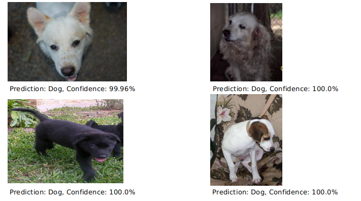
Let’s look at some of the correct and wrong predictions.

Correct Predictions (Dogs)

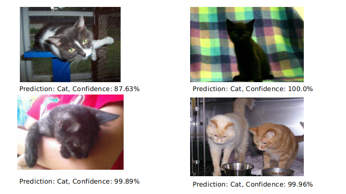
Correct Predictions of Dogs

Correct Predictions (Cats)

Correct Predictions of Cats

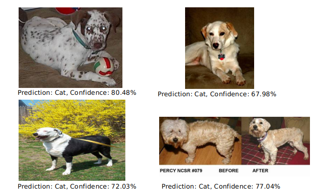
Wrong Predictions (Dogs)

Wrong Predictions of Dogs

Wrong Predictions (Cats)

Wrong Predictions of Cats

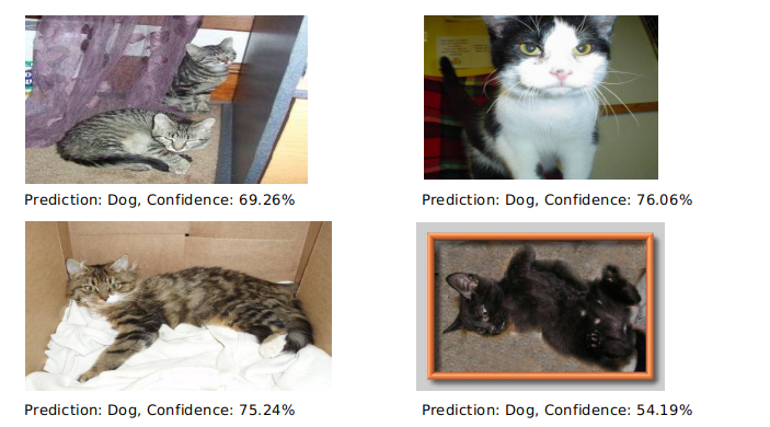
Clearly, the network has done well for just a 2 Convolutional and 3 FC Layer Network. It seems to have focused more on the posture of the animal (and body). We can make the network learn more robust features, with a more deeper CNN (like VGG-16). We’ll be discussing on using pretrained weights on Dogs vs Cats Dataset using PyTorch C++ API and also Transfer Learning Approach in C++.

Happy Learning!